In our last post, we introduced the idea of shrinkage. In this post we are going to extend that idea to improve our results when we segment our data by customer.

Often what we really want is to discover what digital experience is working best for each customer.  A major problem is that as we segment our customers into finer and finer audiences, we have less and less data to use for each segment. In a way segmentation is the opposite of pooling -we want to analyze the data in small chunks, rather than analyzing it as one big blob.

In the previous post we showed how partial-pooling can help improve our estimates of individual items by adjusting them back toward a pooled, or global mean.

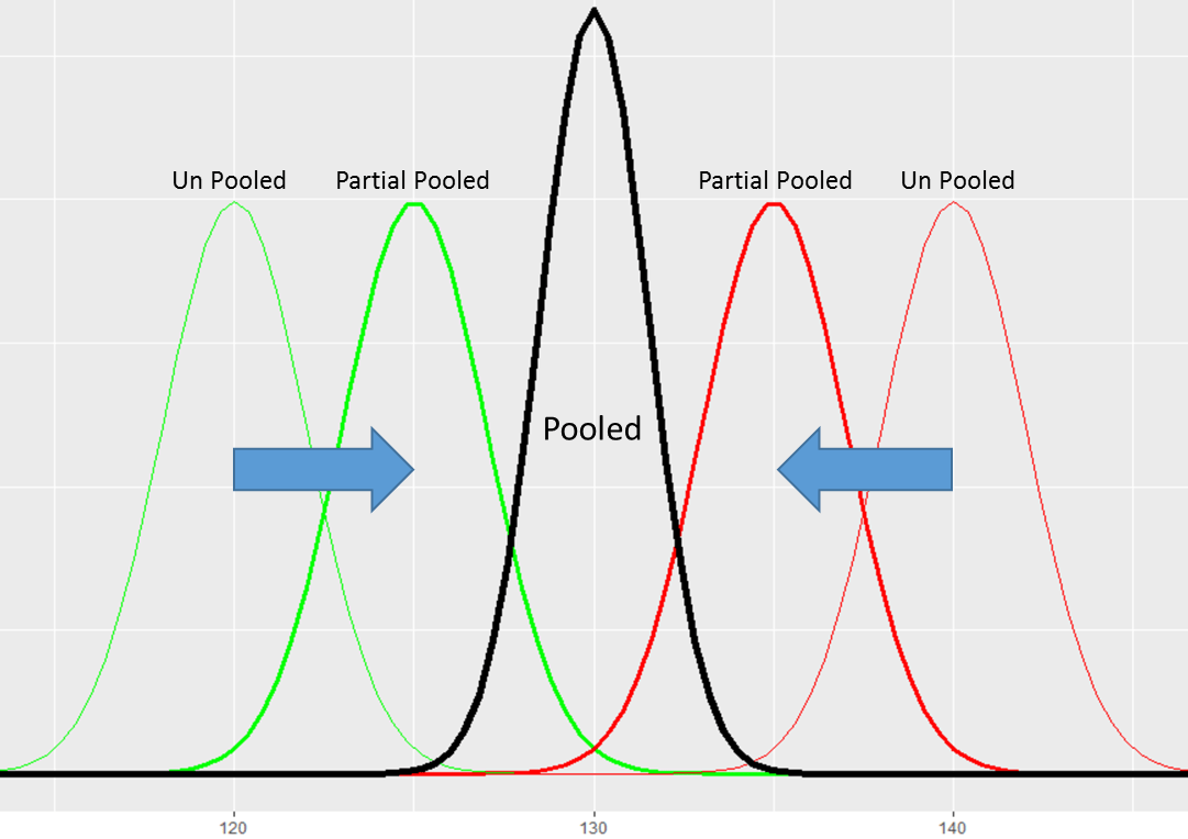
We noted that this is especially effective when we don’t have much data to estimate each individual mean.

Segmentation: Unpooled

For our segmentation use case we will keep it simple and assume we know just two things about our users. They are either a new or repeat customer, and they either live in a rural or suburban neighborhood.

We want to estimate the conversion rate for each test option in our AB Test for each of the four possible user segments (Repeat+Suburban; Repeat+Rural; New+Suburban; New+Rural). This is going to give us eight total conversion rates – two conversion rates for each segment.  So you can see, even in a super simple case, we already have a bunch of individual means we need to estimate.

In our little scenario, the null hypothesis is actually going to be true, so there is no difference in conversion rate between A and B.  In addition, neither of the user features (New/Repeat; Suburban/Rural) will have any impact on conversion rate – they are going to be useless.

We set the conversion rate for both A and B to be 20% (0.2) and then draw 100 random samples and we get the following results:

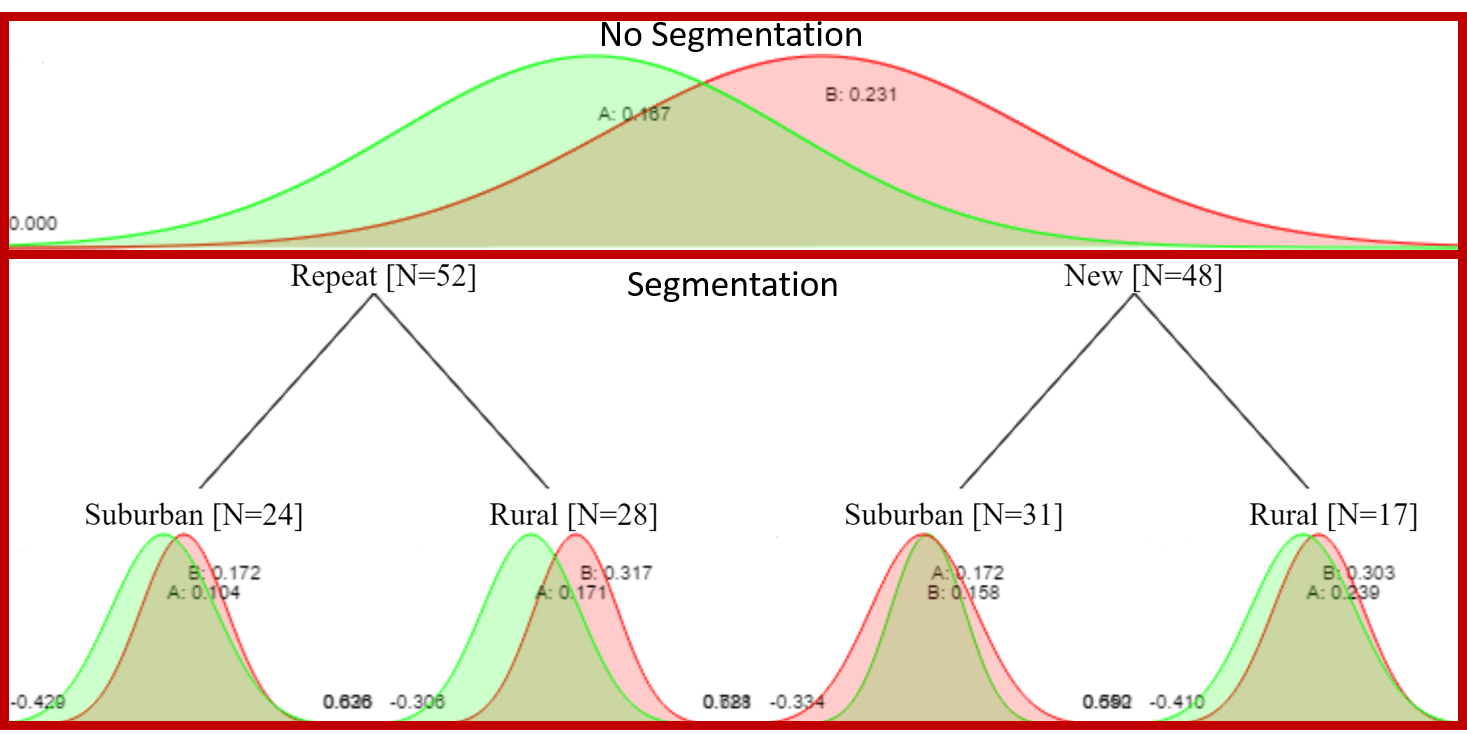
The unsegmented conversion rates are A=16.7% and B=23.1%.  If we just stopped at 100 observations, we would find that B has a 78% probability of being better than A. Not conclusive by any means, but might be enough to lead some astray in to concluding that B is best.

When we segment our results, we find the conversion rates are all all over the place:
1) Repeat+Suburban A=10.4%, B=17.2%; Probability B is best 72%
2) Repeat+Rural A=17.1%, B=31.7%; Probability B is best 88%
3) New+Suburban A=17.2%, B=15.8%; Probability B is best 49%
4) New+Rural A=23.9%,B=30.3%; Probability B is best 51%

Just looking at these numbers we might be tempted to think that Rural customers have higher conversion rates and that option B is probably best for Repeat+Rural customers .

Remember, the real conversion rate for both options, A and B, regardless of segment is 20%.

Segmentation: Partial Pooling

Now lets rerun our simulation, but this time we will calculate the partial pooled values by shrinking our option results back to the grand/pooled average.

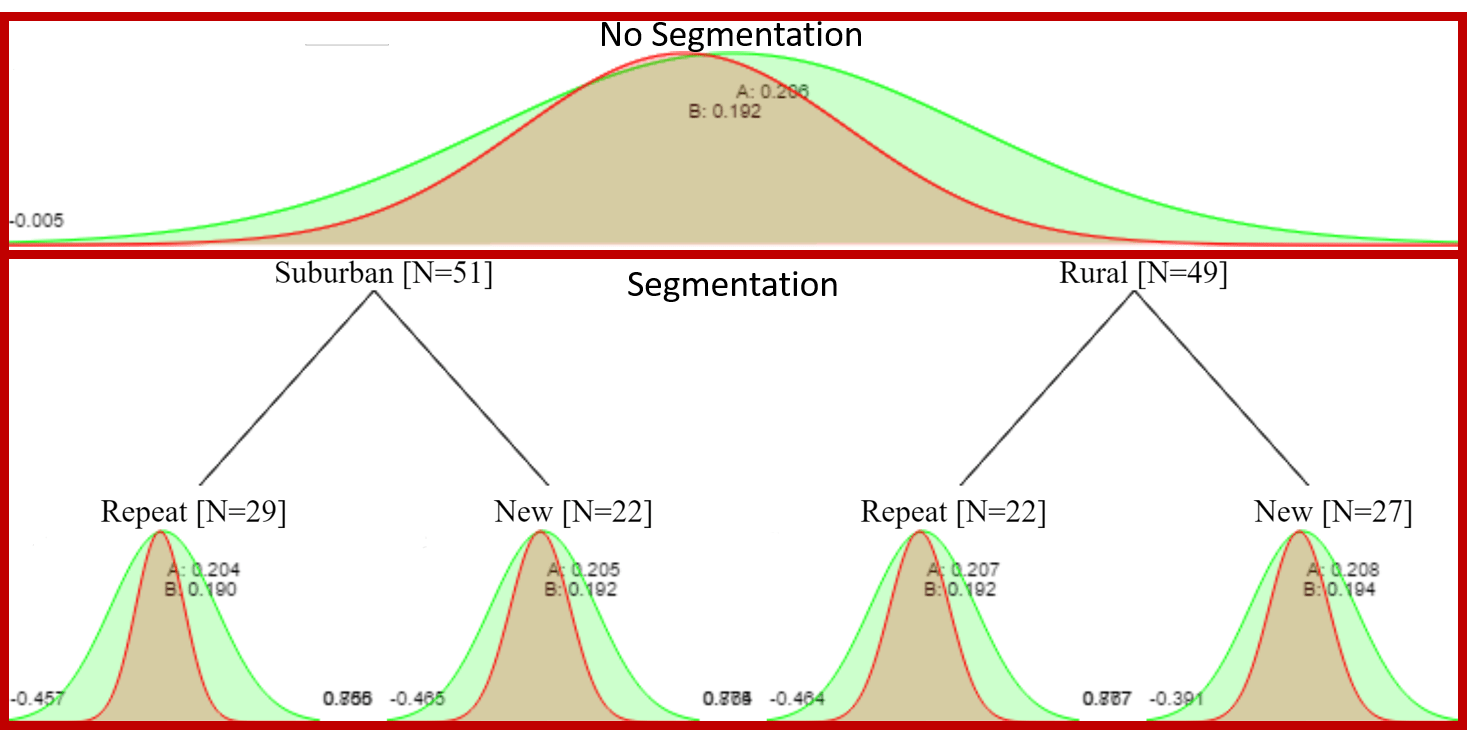
Notice that our unsegmented A and B estimates are pulled toward 20%, with A=20.6% and B=19.2%. After 100 trials, the probability that A is best is just 60%.

We can add another level of partial pooling by shrinking each of the segment results back toward the respective option mean:
1) Repeat+Suburban A=20.4%, B=19.0%
2) Repeat+Rural A=20.7%, B=19.2%
3) New+Suburban A=20.5%, B=19.2%
4) New+Rural A=20.8%,B=19.4%

Now, each of the options for each segments have a 50%/50% probability to be the best, which is what we would expect given that there really is no difference in the conversion rates.

Just to recap this section. We first shrunk our unsegmented A and B estimates toward the average conversion rate over both options.  Then we used these partial-pooled unsegmented option values as a grand average for the segments, and used them for shrinking the values for the segments.

Shrinkage, Targeting, and Multi-Armed Bandits

Where this really gets useful is when you are running a targeted optimization problem with an adaptive method, such as contextual bandits/RL with function approximation.

With multi-armed bandits, rather selecting options with an equal probability, as we do with AB testing, we can instead make our selections based on the probability that each option is best.  So for example, based on the unpooled results we would select B 88% and A 22% of the time for Repeat+Rural customers.   In this use-case it doesn’t really matter, but as you can imagine in a real world scenario,  any intelligent optimization algorithm will need to sort through hundreds of possible segments, option combinations.  What we don’t want, is to confuse the learning system with all of the noise that is bound to creep in to the results when there are so many combinations under consideration.  By feeding the bandit algorithm the partial pooled estimates, rather than the unpooled, we are able to stabilize the optimization process in early, most uncertain portion of the learning.

Maybe even more valuable, is when we introduce new options into an ongoing optimization effort.  So lets say we added a ‘C’ option.  By using shrinkage, we automatically get a reasonable initial estimate for our new option. We just shrink it to the current grand mean of the problem, which is almost certainly a better initial guess then zero. This way the new option has a better chance of being selected by our bandit method (where we make draws from the posterior distributions).

If you would like to learn more about how Conductrics blends partial pooling, predictive targeting, testing, and bandits, please reach out.