A few weeks ago I was talking with Kelly Wortham during her excellent
AB Testing webinar series. During the conversation, one of the attendees asked if they just wanted to pick between A and B, did they really need to run standard significance tests at a 90% or 95% confidence levels?
The simple answer is no. In fact, in certain cases, you can avoid dealing with p-values (or priors and posteriors) altogether and just pick the option with the highest conversion rate.
Even more interesting, at least to me, is that simple approach can be viewed as either form of classical hypothesis testing or as an epsilon- first solution to the multi-arm bandit problem.
Before we get into our simple testing trick, it might be helpful to first revisit a few important concepts that underpin why we are running tests in the first place.
The reason we run experiments is to help determine how different marketing interventions will affect the user experience. The more data we collect, the more information we have, which reduces our uncertainty about the effectiveness of each possible intervention. Since data collection is costly, the question that always comes up is ‘how much data do I really need to collect?’
In a way, every time we run an experiment, we are trying the balance the following: 1) the cost of making a Type 1 error; 2) the cost of making a Type 2 error; and 3) the cost of data collection to help reduce our risk of making either of these errors.
To help answer this question, I find it helpful to organize optimization problems into two high level classes of problems:
1) Do No Harm
These are problems where there is either:
- an existing process, or customer experience, that the organization is counting on for at least a certain minimum level of performance.
- a direct cost associated with implementing a change.
For example, while it would be great if we could increase conversions from an existing check out process, it may be catastrophic if we accidentally reduced the conversion rate. Or, perhaps we want to use data for targeting offers, but there is a real direct cost we have to pay in order to use the targeting data. If it turns out that there is no benefit to the targeting, we will incur the additional data cost without any upside, resulting in a net loss.
So, for the ‘Do No Harm’ type of problem we want to be pretty sure that if we do make a change, it won’t make things worse. For these problems we want to stay the current course unless we have strong evidence to take an alternative action.
2) Go For It
In the ‘Go For It’ type of problem there often is no existing course to follow. Here we are selecting between two or more novel choices AND we have symmetric costs, or loss, if we make a Type I error (reviewed below).
A good example is headline optimization for news articles. Each news article is, by definition, novel, as are the associated headlines. Assuming that one has already decided to run headline optimization (which is itself a ‘Do No Harm’ question), there is no added cost, or risk to selecting one or the other headlines when there is no real difference in the conversion metric between them. The objective of this type of problem is to maximize the chance of finding the best option, if there is one. If there isn’t one, then there is no cost or risk to just randomly select between them (since they perform equally as well and have the same cost to deploy). As it turns out, Go For It problems are also good candidates for Bandit methods.
State of the World
Now that we have our two types of problems defined, we can ask under what situations we might find ourselves when we finally make a decision (i.e. select ‘A’ or ‘B’). There are two possible states of the world when we make our decisions:
- There isn’t the expected effect/difference between the options
- There is the expected effect/difference between the options
It is important to keep in mind that in almost all cases we won’t be entirely certain what the true state of the world is, even after we run our experiment (you can thank David Hume for this). This is where our two error types, Type I and Type II come into play. You can think of these two error types as really just two situations where our Beliefs about the world are not consistent with the true state of the world.
A Type I error is when we pick the alternative option (the ‘B’ option), because we mistakenly believe the true state of the world is ‘Effect’. Alternatively, a Type II error is when we pick ‘A’ (stay the course), thinking that there is no effect, when the true state of the world is ‘Effect’.
The difference between the ‘Do No Harm’ and ‘Go For It’ problems is in how costly it is to make a Type I error.
The table below is the payoff matrix for each error for ‘Do No Harm’ problems
Payoff: Do No Harm The True State of the World (unknown)
| Decision |
Expected Effect |
No Expected Effect |
| Pick A |
Opportunity Costs |
No Cost |
| Pick B |
No Opportunity Cost |
Cost |
Notice, that if we pick B when there is no effect, we make a Type I error and suffer a cost. Now lets look at the payoff table for the ‘Go For It’ problem.
Payoff: Go For It The True State of the World (unknown)
| Decision |
Expected Effect |
No Expected Effect |
| Pick A |
Opportunity Costs |
No Cost |
| Pick B |
No Opportunity Cost |
No Cost |
Notice that the payoff tables for Do No Harm and Go For It are the same when the true state of the world is that there is an effect. But, they differ when there is no effect. When there is no effect, there is NO relative cost in selecting either A or B.
Why is this way of thinking about optimization problems useful?
Because this can help with what type of approach to take based on the problem.
In the Do No Harm problem we need to be mindful about Type I errors, because they are costly, so we need to factor in the risk of making them when we design our experiments. Managing this risk is exactly what classical hypothesis testing does.
That is why for ‘Do No Harm’ problems, it is best practice to run a classic, robust, AB Test. This is because we care more about minimizing our risk of doing harm (the cost of Type I error) than any benefit we might get from rushing through the experiment (cost of information).
However, it also means that if we have a ‘Go For It’ problem, if there is no effect, we don’t really care how we make our selections. Picking randomly when there is no effect is fine, as each of the options have the same value. It is this case where our simple test of just picking the highest value option makes sense.
Go For It: Tests with no P-Values
Finally we can get to the simple, no p-value test. This test guarantees that if there is a true difference of the minimum discernible effect (MDE), or larger, one will choose the better-performing arm X% of the time, where X is the power of the test.
Here are the steps:
1) Calculate the sample size
2) Collect the data
3) Pick whichever option has the highest raw conversion value. If a tie, flip a coin.
Calculate the sample size almost exactly the same as in a standard test: 1) pick a minimum detectable effect (MDE) – this is our minimum desired lift; 2) select the power of the test.
Ah, I hear you asking ‘What about the alpha, don’t we need to select a confidence level?’ Here is the trick. We want to select randomly when there is no effect. By setting alpha to 0.5, the test Reject the null 50% of the time when null is true (no effect).
Lets go through a simple example to make this clear. Lets say your landing page tends to have a conversion rate of around 4%. You are trying out a new alternative offer, and a meaningful improvement for your business would a lift to a 5% conversion rate. So the minimum detectable effect (MDE) for the test is 0.01 (1%).
We then estimate the sample size needed to find the MDE if it exists. Normally, we pick an alpha of 0.05 , but now we are instead going to use an alpha of 0.5. The final step is to pick the power of the test, lets use a good one, 0.95 (often folks pick, 0.8, but for this case we will use 0.95).
You can use now use your favorite sample size calculator (for Conductrics users this is part of the set up work flow).
If you use R, this will look something like:
power.prop.test(n = NULL, p1 = 0.04, p2 = 0.05, sig.level = 0.5, power = .95,
alternative =”one.sided”, strict = FALSE)
This gives us a sample size of 2,324 per option, or 4,648 in total. If we were to run this test with a confidence of 95% (alpha=0.05) would need to have almost four times the traffic, 9,299 per options, or 18,598 in total.
The following is a simulation of 100K experiments, were each experiment selected each arm 2,324 times. The conversion rate for B was set to 5% and 4% for A. The chart below plots the difference in the conversion rates between A and B. Not surprisingly, it is centered on the true difference of 0.01. The main thing to notice, is that if we pick the option with the highest conversion rate we pick B 95% of the time, which is exactly the power we used to calculate the sample size!
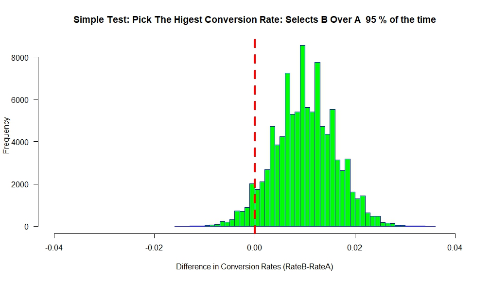
Notice – no p-values, just a simple rule to pick whatever is performing best, yet we still get all of our power goodness! And we only needed about a fourth of the data to reach that power.
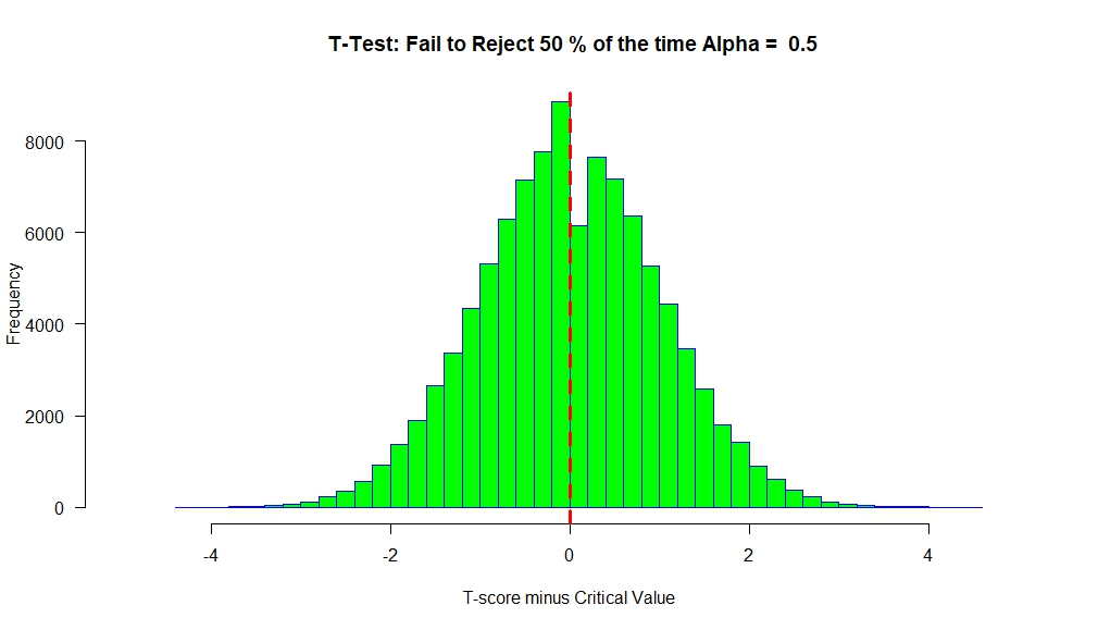
Now lets see what our simulation looks like when both A and B have the same conversion rate of 4% (Null is true).
Notice that the difference between A and B is centered at ‘0’, as we would expect. Using our simple decision rule, we pick B 50% of the time and A 50% of the time.
Now, if we had a Do No Harm problem, this would be a terrible way to make our decisions because half the time we would select B over A and incur a cost. So you still have to do the work and determine your relative costs around data collection, Type 1, Type II errors.
While I was doing some research on this, I came across Georgi Z. Georgiev’s
Analytics tool kit. It has a nice calculator that lets you select your optimal risk balance between there three factors. He also touches on running tests with an alpha of 0.5 in this blog post. Go check it out.
What about Bandits?
As I mentioned above, we can also think of our Go For It problems as a bandit. Bandit solutions that first randomly collect data and then apply the ‘winner’ are known as epsilon-first (To be fair, all AB Testing for decision making can be thought of as Epsilon-first). Epsilon stands for how much of your time you spend during the data collection phase. In this way of looking at the problem, the sample size output from our sample size calculation (based on MDE and Power), is our Epsilon – how long we let the bandit collect data in order to learn.
What is interesting, is that at least in the two option case, this easy method gives us roughly the same results an adaptive Bandit method will. Google has a nice blog
post on Thompson Sampling, which is a near optimal way to dynamically solve bandit problems. We also use
Thompson Sampling here at Conductrics, so I thought it might be interesting to compare their results on the same problem.
In one example, they run a Bandit with two arms, one with a 4% conversion rate, and the other with a 5% conversion rate – just like our example. While they show the Bandit performing well, needing only an average of 5,120 samples, you will note that that is still slightly higher than the fixed amount we used (4,648 samples) in our super simple method.
This doesn’t mean that we don’t ever want to use Thompson Sampling for bandits. As we increase the number of possible options, and many of those options are strictly worse than the others, running Thompson Sampling or another adaptive design can make a lot of sense. (That said, by using a multiple comparison adjustments, like the Šidák correction, I found that one can include K>2 arms in the simple epsilon-first method and still get Type 2 power guarantees. But, as I mentioned, this becomes a much less competitive approach if there are arms that are much worse than the MDE.)
The Weeds
You may be hesitant to believe that such a simple rule can accurately help detect an effect. I checked in with Alex Damour, the Neyman Visiting Assistant Professor over at UC Berkeley and he pointed out that this simple approach is equivalent to running a standard t-test of the following form. From Alex:
“Find N such that P(meanA-meanB < 0 | A = B + MDE) < 0.05. This is equal to the N needed to have 95% power for a one-sided test with alpha = 0.5.
Proof: Setting alpha = 0.5 sets the rejection threshold at 0. So a 95% power means that the test statistic is greater than zero 95% of the time under the alternative (A = B + MDE). The test statistic has the same sign as meanA-meanB. So, at this sample size, P(meanA – meanB > 0 | A = B + MDE) = 0.95.”
To help visualize this, we an rerun our simulation, but run our test using the above formulation.
Under the Null (No Effect) we have the following result
We see that the T-scores are centered around ‘0’. At alpha=0.5, the critical value will be ‘0’. So any T-score greater than ‘0’ will lead to a ‘Rejection’ of the null.
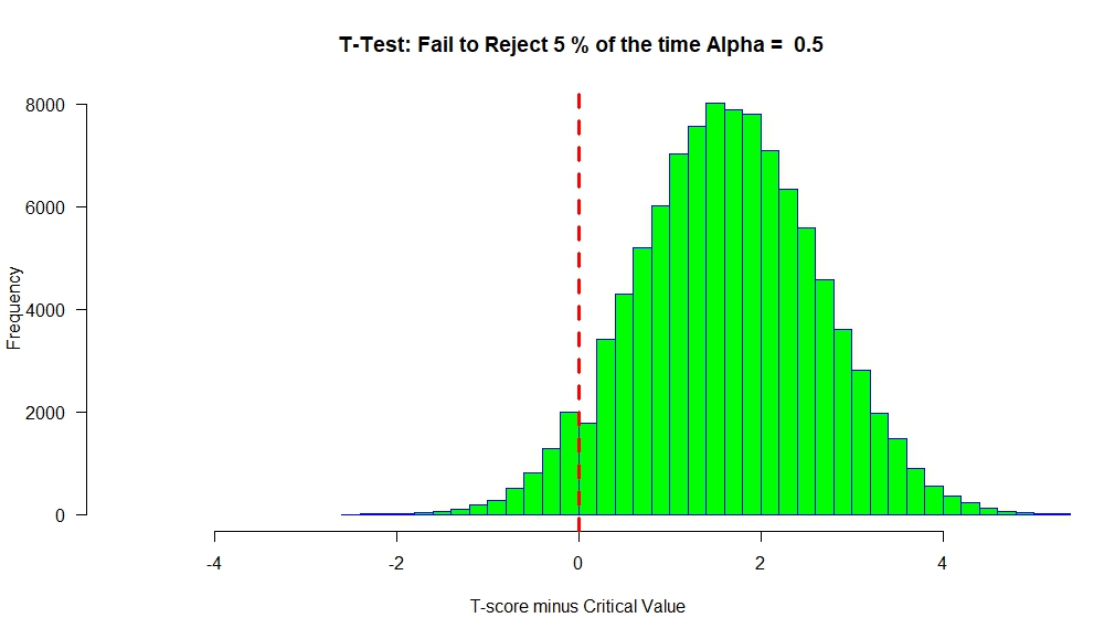
If there is an effect, then we get the following result.
Our distribution of T-scores is shifted to the right, such that only 5% of them (on average) are below ‘0’.
A Few Final Thoughts
Interestingly, at least to me, is that the alpha=0.5 way to solve the ‘Go For It’ problems straddles two of our main approaches in our optimization toolkit. Depending how you look at it, it can be seen as either: 1) A standard t-test (albeit one with the critical value set to ‘0’); or 2) as an epsilon-first approach to solve a multi-arm bandit.
Looking at it this way, the ‘Go For It’ way of thinking about optimization problems can help bridge our understanding between the two primary ways of solving our optimization problems. It also hints that as one moves away from Go For It into Do No Harm (higher Type 1 costs), perhaps classic, robust hypothesis testing is the best approach. As we move toward Go For It, one might want to rethink the problem as a multi-arm bandit.
Have fun, don’t get discouraged, and remember optimization is HARD – but that is what makes all the effort required to learn worth it!


5 Comments
The key point about about A/B testing not mentioned is GENERALIZATIONS. When you run many experiments, you want to learn to generalize. When you just ship low confidence winners, it’s hard to generalize the learnings. Even in go-for-it scenarios like picking between two news article titles, there’s room to learn which style of headlines works better.
Thanks for the comment Ronny. Yep, of course there are many different use cases for running experiments. I wouldn’t suggest using this simple approach for most problems. I do think that it is interesting that by just appealing to the NP-lemma, and then using a trivial decision rule one can get similar results (at least in the simple two arm cases) to near optimal bandit methods (optimal wrt regret).
Nice job! This post is great at explaining that not all tests are equal towards risk management.
But I found it quite complex to explain to non data-scientist people, this is due to the pValue concept which is counter intuitive.
Why don’t you explain this idea in a Bayesian framework ?
The provided confidence interval around the lift, is a more intuitive way to understand risk/gain trade off.
Hi Hubert – thanks for the kind words.
Re Bayesian: I did run some simulations using MC comparisons of the predicted posterior distributions of each arm. I didn’t include them bc: 1) I felt that the post was already pretty dense; 2) We are really asking a frequentist question here (I think it is fair to say we are implicitly invoking the Neyman-Pearson lemma); 3) I wasn’t sure what Bayesian framework to use – I was just estimating the probability that B>A, but I guess one could argue a Bayesian framework should use Bayes Factors (BF). I think that introducing BFs would just muddy the waters more.
I guess I could have another short post, and just walk through the results of the Posterior simulations – but again, since we are asking a freq question, the results don’t really differ, but maybe that would be of interest.
Putting aside the question of what is the goal of experimentation – yes/no decisions or estimation, I think the above approach has several issues.
First, it is not “without p-values”. It uses a p-value of 0.5, just as Prof. Damour confirms in the article itself.
Once we have that down, it becomes clear that type I and type II are reversed – type I > type II. Type I should be the error we most want to avoid, type II should be a less severe error, so the hypotheses should be defined such that Type I B”, while the alternative covers “A <= B". Thus we explicitly state that the error we want to avoid the most is "failure to implement a superior solution", not the usual "implementing a non-superior solution". I'm not sure many people would subscribe to such an approach for obvious reasons.
I have written about non-inferiority tests which are suitable in situations called "go for it" above, and "easy decisions" in my work. In it, however, the primary error is changed from "implementing a non-superior solution" to "implementing an inferior solution", which I believe better addresses the scenario posed in the article.
The major issue with the proposed approach is that when viewed from the point of balancing risk and reward, I could not identify sample size (duration), prior expectation of the result and duration of exploitation of the test outcome, in which using 50% significance and 95% power as defined above, is optimal. Not even an unrealistic one. There could be one, but despite my efforts, I could not find a situation in which using this rule leads to a risk/reward ratio that is optimal. I've used my A/B testing ROI calculator to calculate the risk and reward with $0 costs to perform the test itself, $0 implementation, $0 maintenance costs, and a symmetrical prior distribution for the expected effect, reflecting the "go for it" scenario. If anyone has a better idea of how to calculate risk and reward, I'd be happy to see it.
The claim ""…we still get all of our power goodness! And we only needed about a fourth of the data to reach that power." can be misleading. Since power is derived from the significance threshold and sample size, claiming that you reach the same power level with a lower sample size is not warranted. Power is defined as probability to detect a true effect at a given significance level. Drop significance from 95% to 50% and having 95% power is not the same as having 95% power. It becomes an apples to oranges comparison.
"This test guarantees that if there is a true difference of the minimum discernible effect (MDE), or larger, one will choose the better-performing arm X% of the time, where X is the power of the test." – should be modified slightly to avoid confusion: either drop the "or larger" part, or replace "arm X% of the time" with "arm at least X% of the time".