As some of you may have noticed, there are often little skirmishes that occasionally break out in digital testing and optimization. There are the AB test vs multi-armed bandits debate (both are good, depending on task), standard vs multivariate testing (same, both good), and the Frequentist vs. Bayesian testing argument (also, both good). In the spirit of bringing folks together, I want to introduce the concept of shrinkage. It has Frequentist and Bayesian interpretations, and is useful in both sequential, Bayesian, and bandit style testing. It is also useful for building predictive models that work better in the real world.

Before we get started talking about shrinkage, lets first step back and revisit our coffee example from our post on P-Values (http://blog.conductrics.com/pvalues).  In one of our examples, we wanted to know which place in town has the hotter coffee: McDonald’s or Starbucks.  In order to answer that, we needed to estimate the average temperatures and variances in temperature for both McDonalds and Starbucks coffees. After we calculated the temperature of our samples of cups of coffee from each store, we got something like this:

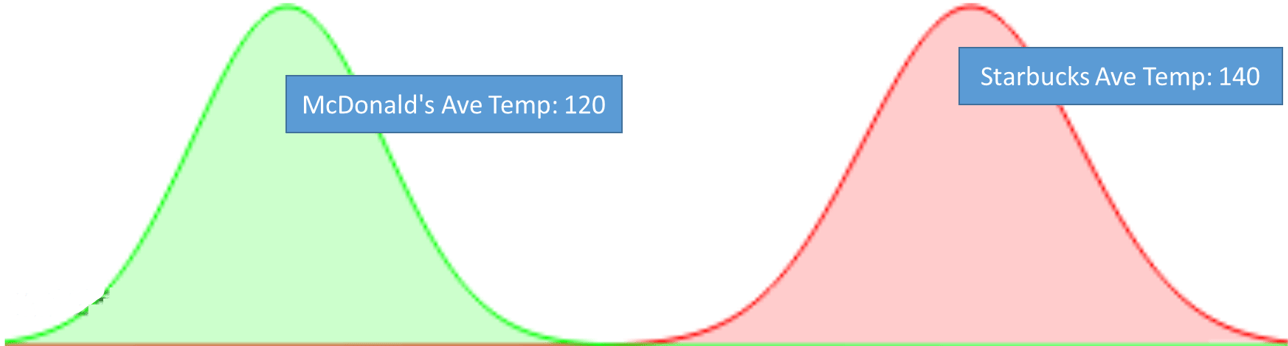
(Perhaps because McDonalds got burned (heh) in the past for serving scalding coffee they are now serving lower average coffee temps than Starbucks.)

In most A/B testing situations we calculate unpooled averages. Unpooled means that we calculate a separate set of statistics based only on the data from each collection.  In our coffee example, we have two collections – Starbucks and McDonald’s. Our unpooled estimates don’t co-mingle the data between stores. One downside of unpooled averages is that each estimated average is based on just a portion of the data. And if you remember, the sampling error (how good/bad our estimate is of the true mean/average) is a function of  how much data we have. So less data means much less certainty around our estimated value.

Data Pooling

We could ignore that the coffee comes from two different stores and pool the data together. Here is what that looks like: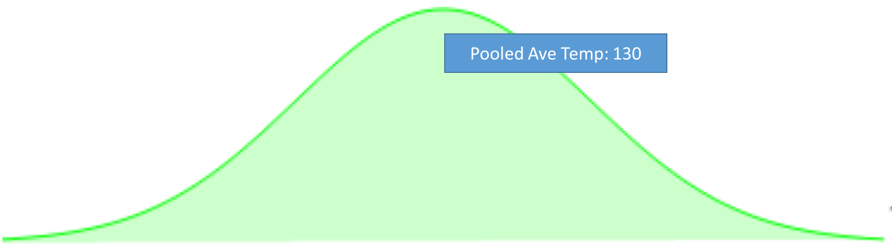

The pooled estimate gives us the grand average temperature for any cup of coffee in town.  You may wonder why this pooled average is interesting to us, since what we really care about is finding the average coffee temperature at each store.

As it turns out we can use our pooled average to help us reduce uncertainty,  in order to get better estimates for each store, especially when have only a small amount of data with which to make our calculations. This often is the case when we have many different collections that we need to come up with individual estimates for.

Partial Pooling

You can think of partial pooling as a way of averaging together our pooled and our unpooled estimates.  This lets us share information across all of the collections, while also being able to estimate individual results.  By using partial pooling, we get the pooled benefit of tapping into all of the coffee data to calculate our store level coffee temperatures, and the unpooled advantage of having a unique temperature value for each store. Since we are effectively averaging the pooled and unpooled values together, this has the effect of pulling each estimated value back toward each other – toward the grand/pooled mean.

When we take our average of the pooled and unpooled values, we factor in how much data we have for each component.  So it is a weighted average. If we have lots of data on the unpooled portion, then we weigh the unpooled estimate more, and the pooled value has very little impact. If, on the other hand, we have very little data for the unpooled estimate, than the pooled value makes up a larger share of our partial pooled estimate.

The pooled value is like the gravitational center of your data. Collections with sparse data don’t have much energy to pull away from that center and get squeezed, or shrunk toward it.

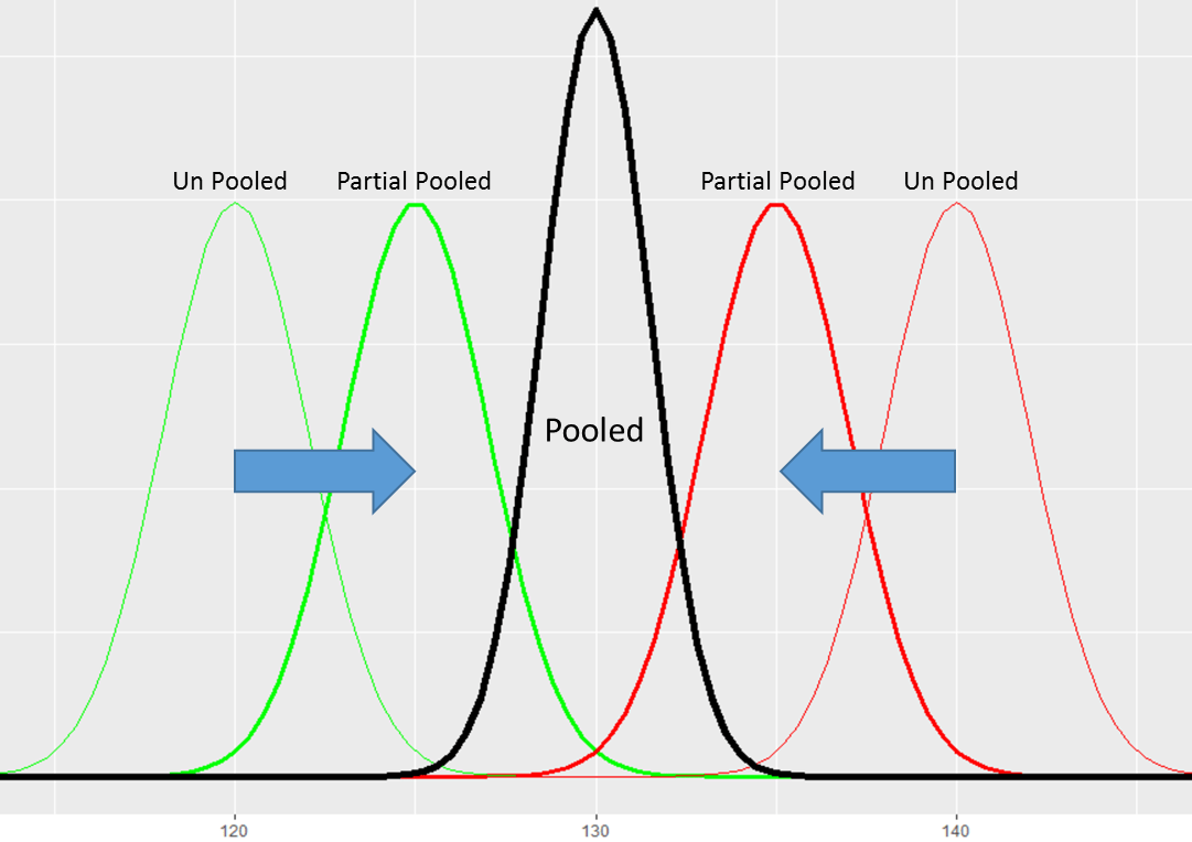
However, as we get more data on each option, the partial pooled values will start to move away from the center value and move toward their unpooled values.

Partial pooling can improve our estimates when we have lots of separate collections we want to estimate and when the collections are in some sense from the same family.

Imagine that instead of two or three coffee shops, we had 50 or even 100 places that sell coffee. We might only be able to sample a handful of cups from each store. Because of our small samples, our unpooled estimates will all be very noisy, with some having very high temps and some very low temps. By using partial pooling we smooth out the noise and pull all of the outliers back toward the grand average.  This tugging-in of our individual results toward the center – called shrinkage – is a tradeoff of bias for less variance (noise) in our results.

If you are not convinced, here is another example. Let’s say we wanted to know the what the average temperature of a cup of coffee is from the town’s local cafe. Even before we test our first cup of coffee, we already have a strong evidence that the temperature will be somewhere around 130 degrees, since the coffee temp of the independent cafe belongs to the family of all coffee shop coffee temperatures. If you then tested a cup of coffee from the cafe, and found it was only 90 F, you might think that while the cafe’s average temperature might be less than average coffee temperature, it is probably higher than 90 F.

Partial Pooling and Optimization

We can use this same idea when we are run sequential, empirical Bayesian, or bandit style tests. By using partial pooling, we help stabilize our predictions in the early stages of a campaign. It also allows us to make reasonable predictions to new options added mid-test.

Shrinking the individual means back to the grand mean is also consistent with the null hypothesis from standard testing – we assume that all of the different test options are drawn from the same distribution.  Partial pooling implicitly includes that assumption directly into the estimated values.  However, as we collect more data, each result moves away from the center. Partial pooled results sit along the continuum between pooled and unpooled estimates. What is nice, is that the data determines where we are on the continuum.

What to learn more about partial pooling and are a Frequentist?  Look up random effects models. If you are Bayesian, please see hierarchical modelling.  And if you are cool with either, see empirical Bayes and James-Stein estimators.

If you want to learn more about how Conductrics uses shrinkage, and how we can help you provide better digital experiences for your customers please reach out.